Urban Scale Example Model

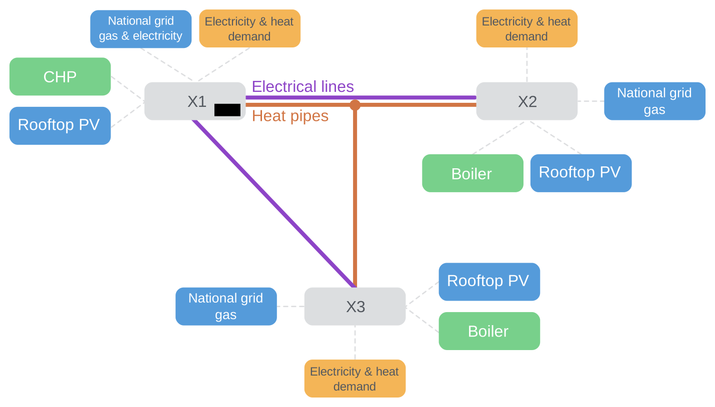
This example consists of two possible sources of electricity, one possible source of heat, and one possible source of simultaneous heat and electricity. There are three locations, each describing a building, with transmission links between them.

The diagram below gives an overview:

Urban scale example model overview

We distinguish between model configuration (the options provided to Calliope to do its work) and the model definition (your representation of a physical system in YAML).

Model configuration

The model configuration file model.yaml is the place to tell Calliope about how to interpret the model definition and how to build and solve your model. It does not contain much data, but the scaffolding with which to construct and run your model.

You will notice that we load a "math" file in config.init. You can find out more about this user-defined math below

config:
  init:
    name: Urban-scale example model
    # What version of Calliope this model is intended for
    calliope_version: 0.7.0
    subset:
      timesteps: ["2005-07-01", "2005-07-02"] # Subset of timesteps
    broadcast_input_data: true  # allow single indexed parameter data entries to be broadcast across all index items, if there are multiple entries.
    math_paths:
      additional_math: "additional_math.yaml"
    extra_math: ["additional_math"]
    mode: base # Choices: base, operate, spores

  build:
    ensure_feasibility: true # Switching on unmet demand

  solve:
    solver: cbc

Bringing the YAML files together

Technically, you could define everything about your model in the same file as your configuration. One file with the top-level keys config, data_definitions, techs, nodes, templates, scenarios, overrides. However, this tends to become unwieldy.

Instead, various parts of the model are defined in different files and then we import them in the YAML file that we are going to load into calliope (calliope.Model("my_main_model_file.yaml")). The import section in our file looks like this:

import: # Import other files from paths relative to this file, or absolute paths
  - "model_config/techs.yaml"
  - "model_config/locations.yaml"
  - "scenarios.yaml"

Model definition

Referencing tabular data

As of Calliope v0.7.0 it is possible to load tabular data completely separately from the YAML model definition. To do this we reference data tables under the data_tables key:

data_tables:
  demand:
    table: data_tables/demand.csv
    rows: timesteps
    columns: [techs, nodes]
    add_dims:
      inputs: sink_use_equals
  pv_resource:
    table: data_tables/pv_resource.csv
    rows: timesteps
    columns: [comment, scaler]
    add_dims:
      inputs: source_use_equals
      techs: pv
    select:
      scaler: per_area
    drop: [comment, scaler]
  export_power:
    table: data_tables/export_power.csv
    rows: timesteps
    columns: nodes
    add_dims:
      inputs: cost_export
      techs: chp
      costs: monetary
      carriers: electricity

In the Calliope urban scale example model, we only load timeseries data from file, including for energy demand, electricity export price and solar PV resource availability. These are large tables of data that do not work well in YAML files! As an example, the data in the energy demand CSV file looks like this:

techs	demand_heat	demand_heat	demand_heat	demand_electricity	demand_electricity	demand_electricity
nodes	X1	X2	X3	X1	X2	X3
2005-01-01 00:00	4.348486	128.210300	25.173941	0.637704	101.809815	20.592169
2005-01-01 01:00	4.516168	106.472403	19.648068	0.523598	101.809815	20.286959

You'll notice that in each row there is reference to a timestep, and in each column to a technology and a node. Therefore, we reference timesteps in our data table rows, and nodes and techs in our data table columns. Since all the data refers to the one parameter sink_use_equals, we don't add that information in the CSV file, but instead add it on as a dimension when loading the file.

Info

You can read more about loading data from file in [our dedicated tutorial][loading-tabular-data].

Data definitions for indexed parameters

Before we dive into the technologies and nodes in the model, we have defined the data for some indexed parameters that are independent of both technologies and nodes:

data_definitions:
  objective_cost_weights:
    data: 1
    index: monetary
    dims: costs
  # `bigM` sets the scale of unmet demand, which cannot be too high, otherwise the optimisation will not converge
  bigM: 1e6
  cost_interest_rate:
    data: 0.10
    index: monetary
    dims: costs

Neither of these parameters is strictly necessary to define. They have defaults assigned to them (see the model definition schema in the reference section of the documentation). However, we have included them in here as examples.

objective_cost_weights can be used to weight different cost classes in the objective function (e.g., if we had co2_emissions as well as monetary costs). bigM (https://en.wikipedia.org/wiki/Big_M_method) is used to formulate certain types of constraints and should be a large number, but not so large that it causes numerical trouble.

bigM is dimensionless, while objective_cost_weights is indexed over the costs dimension. You will see this same parameter definition structure elsewhere in the model definition as we index certain parameters over other dimensions.

Supply technologies

This example model defines three supply technologies.

The first two are supply_gas and supply_grid_power, referring to the supply of gas (natural gas) and electricity, respectively, from the local distribution system. These 'infinitely' available national commodities can become carriers in the system, with the cost of their purchase being considered at supply, not conversion.

The layout of a supply technology which has an infinite source, a carrier conversion efficiency ($flow_{eff}^{out}$), and a constraint on its maximum built $flow_{cap}$ (which puts an upper limit on $flow_{out}$).

The definition of this technology in the example model's configuration looks as follows

supply_grid_power:
  name: "National grid import"
  color: "#C5ABE3"
  base_tech: supply
  carrier_out: electricity
  source_use_max: .inf
  flow_cap_max: 2000
  lifetime: 25
  cost_flow_cap:
    data: 15
    index: monetary
    dims: costs
  cost_source_use:
    data: 0.1 # 10p/kWh electricity price #ppt
    index: monetary
    dims: costs

supply_gas:
  name: "Natural gas import"
  color: "#C98AAD"
  base_tech: supply
  carrier_out: gas
  source_use_max: .inf
  flow_cap_max: 2000
  lifetime: 25
  cost_flow_cap:
    data: 1
    index: monetary
    dims: costs
  cost_source_use:
    data: 0.025 # 2.5p/kWh gas price #ppt
    index: monetary
    dims: costs

The final supply technology is pv (solar photovoltaic power), which serves as an inflexible supply technology. It has a time-varying source availability loaded from CSV, a maximum area over which it can capture its source (area_use_max) and a requirement that all available source is used (source_use_equals). This emulates the reality of solar technologies: once installed, their production matches the availability of solar energy.

The efficiency of the DC to AC inverter (which occurs after conversion from source to carrier) is considered in parasitic_eff. The area_use_per_flow_cap gives a link between the installed area of solar panels to the installed capacity of those panels (i.e. kWp).

In most cases, domestic PV panels are able to export excess energy to the national grid. We allow this here by specifying carrier_export. Revenue for export will be considered on a per-location basis.

The definition of this technology in the example model's configuration looks as follows:

pv:
  name: "Solar photovoltaic power"
  color: "#F9D956"
  base_tech: supply
  carrier_out: electricity
  carrier_export: electricity
  source_unit: per_area
  area_use_per_flow_cap: 7 # 7m2 of panels needed to fit 1kWp of panels
  flow_out_parasitic_eff: 0.85 # inverter losses
  flow_cap_max: 250
  area_use_max: 1500
  lifetime: 25
  cost_flow_cap:
    data: 1350
    index: monetary
    dims: costs

Conversion technologies

The example model defines two conversion technologies.

The first is boiler (natural gas boiler), which serves as an example of a simple conversion technology with one input carrier and one output carrier. Its only constraints are the cost of built capacity (costs.monetary.flow_cap), a constraint on its maximum built capacity (constraints.flow_cap_max), and a carrier conversion efficiency (flow_out_eff).

The layout of a simple conversion technology, in this case `boiler`, which has one carrier input and output, a carrier conversion efficiency ($flow_{eff}^{out}$), and a constraint on its maximum built $flow_{cap}$ (which puts an upper limit on $flow_{out}$).

The definition of this technology in the example model's configuration looks as follows:

boiler:
  name: "Natural gas boiler"
  color: "#8E2999"
  base_tech: conversion
  carrier_in: gas
  carrier_out: heat
  cost_flow_cap:
    data: 30
    index: [[monetary, heat]]
    dims: [costs, carriers]
  flow_cap_max:
    data: 600
    index: heat
    dims: carriers
  flow_out_eff: 0.85
  lifetime: 25
  cost_flow_in:
    data: 0.004 # .4p/kWh
    index: monetary
    dims: costs

There are a few things to note. First, boiler defines a name and a color (given as an HTML color code). These can be used when visualising your results. Second, it specifies its base_tech, conversion, its inflow carrier gas, and its outflow carrier heat, thus setting itself up as a gas to heat conversion technology. This is followed by the definition of constraining parameters and costs; the only cost class used is monetary but this is where other "costs", such as emissions, could be defined.

The second technology is chp (combined heat and power), and serves as an example of a possible conversion_plus technology making use of two output carriers.

The layout of a more complex node which makes use of multiple output carriers.

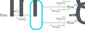
This definition in the example model's configuration is more verbose:

chp:
  name: "Combined heat and power"
  color: "#E4AB97"
  base_tech: conversion
  carrier_in: gas
  carrier_out: [electricity, heat]
  carrier_export: electricity
  flow_cap_max:
    data: 1500
    index: electricity
    dims: carriers
  flow_out_eff:
    data: 0.405
    index: electricity
    dims: carriers
  heat_to_power_ratio: 0.8
  lifetime: 25
  cost_flow_cap:
    data: 750
    index: [[monetary, electricity]]
    dims: [costs, carriers]
  cost_flow_out:
    data: 0.004 # .4p/kWh for 4500 operating hours/year
    index: [[monetary, electricity]]
    dims: [costs, carriers]

Again, chp has the definitions for name, color, base_tech, and carrier_in/out. It has two carriers defined for its outflow. Note the parameter heat_to_power_ratio, which we set to 0.8. We will use this to create a link between the two output carriers. More importantly, it is a custom parameter - Calliope does not come with heat_to_power_ratio pre-defined. Therefore, for now, it will not have any effect - we need to introduce our own math.

In this case, we want to ensure that 0.8 units of heat are produced every time a unit of electricity is produced. Furthermore, while producing these units of energy - both electricity and heat - we want to ensure that gas consumption is only a function of electricity output.

Interlude: user-defined math

The pre-defined Calliope math does not have the capacity to handle our chp technology definition from above. By default, setting two output carriers would mean that the choice is between those technologies (e.g., a heat pump that can produce heat or cooling). To ensure our chp will be constrained as we expect, we add our own math:

parameters:
  heat_to_power_ratio:
    default: 1
    title: Heat to power ratio for CHP
    description: Ratio of heat output to electricity output for combined heat and power (CHP) technology.

constraints:
  link_chp_outputs:
    description: Fix the relationship between heat and electricity output
    foreach: [nodes, techs, timesteps]
    where: "[chp] in techs"
    equations:
      - expression: flow_out[carriers=electricity] * heat_to_power_ratio == flow_out[carriers=heat]

  balance_conversion:
    # Remove the link between CHP inflow and heat outflow (now dealt with in `link_chp_outputs`)
    equations:
      - where: "NOT [chp] in techs"
        expression: sum(flow_out_inc_eff, over=carriers) == sum(flow_in_inc_eff, over=carriers)
      - where: "[chp] in techs"
        expression: flow_out_inc_eff[carriers=electricity] == sum(flow_in_inc_eff, over=carriers)

There are two things we have to do:

1. Create a link between heat and electricity outflow. They both are produced simultaneously. We may prefer to have the heat output be set to a maximum equal to the heat_to_power_ratio, in which case the expression would become:

flow_out[carriers=electricity] * heat_to_power_ratio >= flow_out[carriers=heat]

1. Unlink heat output from gas output. This requires updating a constraint that already exists in the pre-defined math. It is important that you understand the contents of the pre-defined math before you add your own, to ensure you can override the math there appropriately.

Demand technologies

You always need demand for your carriers in a model. These move carriers out of the modelled system and are required for overall energy balance (energy into the system = energy out of the system).

demand_electricity:
  name: "Electrical demand"
  color: "#072486"
  base_tech: demand
  carrier_in: electricity

demand_heat:
  name: "Heat demand"
  color: "#660507"
  base_tech: demand
  carrier_in: heat

Transmission technologies

In this district, electricity and heat can be distributed between nodes. Gas is made available in each node without consideration of transmission.

A transmission technology with the options for flow efficiency ($flow_{eff}^{out}$ and $flow_{eff}^{in}$) and flow capacity ($flow_{cap}$).

X1_to_X2:
  link_from: X1
  link_to: X2
  template: power_lines
  distance: 10
X1_to_X3:
  link_from: X1
  link_to: X3
  template: power_lines
  distance: 5
X1_to_N1:
  link_from: X1
  link_to: N1
  template: heat_pipes
  distance: 3
N1_to_X2:
  link_from: N1
  link_to: X2
  template: heat_pipes
  distance: 3
N1_to_X3:
  link_from: N1
  link_to: X3
  template: heat_pipes
  distance: 4

To avoid excessive duplication in model definition, our transmission technologies inherit most of the their parameters from templates:

power_lines:
  name: "Electrical power distribution"
  color: "#6783E3"
  base_tech: transmission
  carrier_in: electricity
  carrier_out: electricity
  flow_cap_max: 2000
  flow_out_eff: 0.98
  lifetime: 25
  cost_flow_cap_per_distance:
    data: 0.01
    index: monetary
    dims: costs

heat_pipes:
  name: "District heat distribution"
  color: "#823739"
  base_tech: transmission
  carrier_in: heat
  carrier_out: heat
  flow_cap_max: 2000
  flow_out_eff_per_distance: 0.975
  lifetime: 25
  cost_flow_cap_per_distance:
    data: 0.3
    index: monetary
    dims: costs

power_lines has an efficiency of 0.95, so a loss during transmission of 0.05. heat_pipes has a loss rate per unit distance of 2.5%/unit distance (or flow_out_eff_per_distance of 97.5%). Over the distance between the two locations of 0.5km (0.5 units of distance), this translates to \(2.5^{0.5}\) = 1.58% loss rate.

Nodes

In order to translate the model requirements shown in this section's introduction into a model definition, four nodes (i.e. geographic locations) are used: X1, X2, X3, and N1.

The technologies are set up at these nodes as follows:

Nodes and their technologies in the example model.

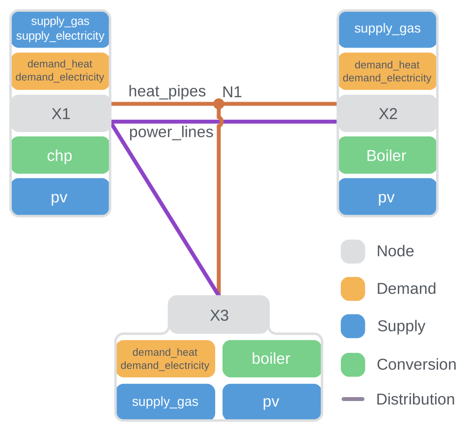
Let's now look at the first location definition:

X1:
  techs:
    chp:
    pv:
    supply_grid_power:
      cost_flow_cap.data: 100 # cost of transformers
    supply_gas:
    demand_electricity:
    demand_heat:
  available_area: 500
  latitude: 51.4596158
  longitude: -0.1613446

There are several things to note here:

• The node specifies a dictionary of technologies that it allows (techs), with each key of the dictionary referring to the name of technologies defined in our techs.yaml file. Technologies listed here must have been defined elsewhere in the model configuration.

• It also overrides some options for both demand_electricity, demand_heat, and supply_grid_power. For grid supply, it sets a node-specific cost. For demands, the options set here are related to reading the demand time series from a CSV file. CSV is a simple text-based format that stores tables by comma-separated rows. We did not define any sink option in the definition of these demands. Instead, this is done directly via a node-specific override.

• Coordinates are defined, but they will not be used for anything in the model as we have already defined the distance along links when we defined our transmission technologies. Coordinates are therefore only useful for geospatial visualisations.

• An available_area is defined, which will limit the maximum area of all area_use technologies to the e.g. roof space available at our node. In this case, we just have pv, but the case where solar thermal panels compete with photovoltaic panels for space, this would limit the sum of the two to the available area.

The remaining nodes look similar:

X2:
  techs:
    boiler.cost_flow_cap.data: 43.1 # different boiler costs
    pv:
      cost_flow_out:
        data: -0.0203 # revenue for just producing electricity
        index: monetary
        dims: costs
      cost_export:
        data: -0.0491 # FIT return for PV export
        index: monetary
        dims: costs
    supply_gas:
    demand_electricity:
    demand_heat:
  available_area: 1300
  latitude: 51.4652373
  longitude: -0.1141548

X3:
  techs:
    boiler.cost_flow_cap.data: 78 # different boiler costs
    pv:
      flow_cap_max: 50 # changing tariff structure below 50kW
      cost_om_annual:
        data: -80.5 # reimbursement per kWp from FIT
        index: monetary
        dims: costs
    supply_gas:
    demand_electricity:
    demand_heat:
  available_area: 900
  latitude: 51.4287016
  longitude: -0.1310635

X2 and X3 are very similar to X1, except that they do not connect to the national electricity grid, nor do they contain the chp technology. Specific pv cost structures are also given, emulating e.g. commercial vs. domestic feed-in tariffs.

N1 differs to the others by virtue of containing no technologies. It acts as a branching station for the heat network, allowing connections to one or both of X2 and X3 without double counting the pipeline from X1 to N1:

N1: # node for branching heat transmission network
  techs:
  latitude: 51.4450766
  longitude: -0.1247183

Revenue by export

You will have seen that both the chp and pv technologies define an export carrier (carrier_export). This means they can export their produced electricity directly out of the system as well as using it to meet demands within the system. Since export "cost" is a negative value for both technologies, they can accrue revenue by exporting electricity.

The revenue from PV export varies depending on location, emulating the different feed-in tariff structures that might exist between e.g. commercial and domestic properties. In domestic properties, the revenue is generated by simply having the installation (per kW installed capacity), as export is not metered. Export is metered in commercial properties, thus revenue is generated directly from export (per kWh exported). The revenue generated by CHP depends on the electricity grid wholesale price per kWh, being 80% of that. Therefore, the export "cost" for CHP is loaded from a CSV file of time-varying values. These revenue possibilities are reflected in the technologies' and locations' definitions.

---

Where to go next

To try loading and solving the model yourself, move on to the accompanying notebook [here][running-the-urban-scale-example-model]. You can also find a list of all the example models available in Calliope here.